uczenie-maszynowe/wyk/06_Problem_nadmiernego_dopasowania.ipynb

Uczenie maszynowe

6. Problem nadmiernego dopasowania

6.1. Regresja wielomianowa

Wprowadzenie: wybór cech

Niech naszym zadaniem będzie przewidzieć cenę działki o kształcie prostokąta.

Jakie cechy wybrać?

Możemy wybrać dwie cechy:

• $x_1$ – szerokość działki, $x_2$ – długość działki: $$ h_{\theta}(\vec{x}) = \theta_0 + \theta_1 x_1 + \theta_2 x_2 $$

...albo jedną:

• $x_1$ – powierzchnia działki: $$ h_{\theta}(\vec{x}) = \theta_0 + \theta_1 x_1 $$

Można też zauważyć, że cecha „powierzchnia działki” powstaje przez pomnożenie dwóch innych cech: długości działki i jej szerokości.

Wniosek: możemy tworzyć nowe cechy na podstawie innych poprzez wykonywanie na nich różnych operacji matematycznych.

Regresja wielomianowa

W regresji wielomianowej będziemy korzystać z cech, które utworzymy jako potęgi cech wyjściowych.

# Przydatne importy

import ipywidgets as widgets
import matplotlib.pyplot as plt
import numpy as np
import pandas

%matplotlib inline

# Przydatne funkcje


def cost(theta, X, y):
    """Wersja macierzowa funkcji kosztu"""
    m = len(y)
    J = 1.0 / (2.0 * m) * ((X * theta - y).T * (X * theta - y))
    return J.item()


def gradient(theta, X, y):
    """Wersja macierzowa gradientu funkcji kosztu"""
    return 1.0 / len(y) * (X.T * (X * theta - y))


def gradient_descent(fJ, fdJ, theta, X, y, alpha=0.1, eps=10**-5):
    """Algorytm gradientu prostego (wersja macierzowa)"""
    current_cost = fJ(theta, X, y)
    logs = [[current_cost, theta]]
    while True:
        theta = theta - alpha * fdJ(theta, X, y)
        current_cost, prev_cost = fJ(theta, X, y), current_cost
        if abs(prev_cost - current_cost) > 10**15:
            print("Algorithm does not converge!")
            break
        if abs(prev_cost - current_cost) <= eps:
            break
        logs.append([current_cost, theta])
    return theta, logs


def plot_data(X, y, xlabel, ylabel):
    """Wykres danych (wersja macierzowa)"""
    fig = plt.figure(figsize=(16 * 0.6, 9 * 0.6))
    ax = fig.add_subplot(111)
    fig.subplots_adjust(left=0.1, right=0.9, bottom=0.1, top=0.9)
    ax.scatter([X[:, 1]], [y], c="r", s=50, label="Dane")

    ax.set_xlabel(xlabel)
    ax.set_ylabel(ylabel)
    ax.margins(0.05, 0.05)
    plt.ylim(y.min() - 1, y.max() + 1)
    plt.xlim(np.min(X[:, 1]) - 1, np.max(X[:, 1]) + 1)
    return fig


def plot_fun(fig, fun, X):
    """Wykres funkcji `fun`"""
    ax = fig.axes[0]
    x0 = np.min(X[:, 1]) - 1.0
    x1 = np.max(X[:, 1]) + 1.0
    Arg = np.arange(x0, x1, 0.1)
    Val = fun(Arg)
    return ax.plot(Arg, Val, linewidth="2")

# Wczytanie danych (mieszkania) przy pomocy biblioteki pandas

alldata = pandas.read_csv(
    "data_flats.tsv", header=0, sep="\t", usecols=["price", "rooms", "sqrMetres"]
)
data = np.matrix(alldata[["sqrMetres", "price"]])

m, n_plus_1 = data.shape
n = n_plus_1 - 1
Xn = data[:, 0:n]
Xn /= np.amax(Xn, axis=0)
Xn2 = np.power(Xn, 2)
Xn2 /= np.amax(Xn2, axis=0)
Xn3 = np.power(Xn, 3)
Xn3 /= np.amax(Xn3, axis=0)

X = np.matrix(np.concatenate((np.ones((m, 1)), Xn), axis=1)).reshape(m, n + 1)
X2 = np.matrix(np.concatenate((np.ones((m, 1)), Xn, Xn2), axis=1)).reshape(m, 2 * n + 1)
X3 = np.matrix(np.concatenate((np.ones((m, 1)), Xn, Xn2, Xn3), axis=1)).reshape(
    m, 3 * n + 1
)
y = np.matrix(data[:, -1]).reshape(m, 1)

Postać ogólna regresji wielomianowej:

$$ h_{\theta}(x) = \sum_{i=0}^{n} \theta_i x^i $$

# Funkcja regresji wielomianowej


def h_poly(Theta, x):
    """Funkcja wielomianowa"""
    return sum(theta * np.power(x, i) for i, theta in enumerate(Theta.tolist()))


def polynomial_regression(theta):
    """Funkcja regresji wielomianowej"""
    return lambda x: h_poly(theta, x)

Najprostszym przypadkiem regresji wielomianowej jest funkcja kwadratowa:

Funkcja kwadratowa:

$$ h_{\theta}(x) = \theta_0 + \theta_1 x + \theta_2 x^2 $$

fig = plot_data(X2, y, xlabel="x", ylabel="y")
theta_start = np.matrix([0, 0, 0]).reshape(3, 1)
theta, logs = gradient_descent(cost, gradient, theta_start, X2, y)
plot_fun(fig, polynomial_regression(theta), X)

[<matplotlib.lines.Line2D at 0x7f737ce1baf0>]

Innym szczególnym przypadkiem regresji wielomianowej jest funkjca sześcienna:

Funkcja sześcienna:

$$ h_{\theta}(x) = \theta_0 + \theta_1 x + \theta_2 x^2 + \theta_3 x^3 $$

fig = plot_data(X3, y, xlabel="x", ylabel="y")
theta_start = np.matrix([0, 0, 0, 0]).reshape(4, 1)
theta, _ = gradient_descent(cost, gradient, theta_start, X3, y)
plot_fun(fig, polynomial_regression(theta), X)

print(theta)

[[ 397519.38046962]
 [-841341.14146733]
 [2253713.97125102]
 [-244009.07081946]]

Regresję wielomianową można potraktować jako szczególny przypadek regresji liniowej wielu zmiennych:

$$ h_{\theta}(x) = \theta_0 + \theta_1 x + \theta_2 x^2 + \theta_3 x^3 $$ $$ x_1 = x, \quad x_2 = x^2, \quad x_3 = x^3, \quad \vec{x} = \left[ \begin{array}{ccc} x_0 \\ x_1 \\ x_2 \end{array} \right] $$

(W tym przypadku za kolejne cechy przyjmujemy kolejne potęgi zmiennej $x$).

Uwaga praktyczna: przyda się normalizacja cech, szczególnie skalowanie!

Do tworzenia cech „pochodnych” możemy używać nie tylko potęgowania, ale też innych operacji matematycznych, np.:

$$ h_{\theta}(x) = \theta_0 + \theta_1 x + \theta_2 \sqrt{x} $$ $$ x_1 = x, \quad x_2 = \sqrt{x}, \quad \vec{x} = \left[ \begin{array}{ccc} x_0 \\ x_1 \end{array} \right] $$

Jakie zatem cechy wybrać? Najlepiej dopasować je do konkretnego problemu.

Wielomianowa regresja logistyczna

Podobne modyfikacje cech możemy również stosować dla regresji logistycznej.

def powerme(x1, x2, n):
    """Funkcja, która generuje n potęg dla zmiennych x1 i x2 oraz ich iloczynów"""
    X = []
    for m in range(n + 1):
        for i in range(m + 1):
            X.append(np.multiply(np.power(x1, i), np.power(x2, (m - i))))
    return np.hstack(X)

# Wczytanie danych
import pandas
import numpy as np

alldata = pandas.read_csv("polynomial_logistic.tsv", sep="\t")
data = np.matrix(alldata)

m, n_plus_1 = data.shape
n = n_plus_1 - 1
Xn = data[:, 1:]

Xpl = powerme(data[:, 1], data[:, 2], n)
Ypl = np.matrix(data[:, 0]).reshape(m, 1)

data[:10]

matrix([[ 1.        ,  0.36596696, -0.11214686],
        [ 0.        ,  0.4945305 ,  0.47110656],
        [ 0.        ,  0.70290604, -0.92257983],
        [ 0.        ,  0.46658862, -0.62269739],
        [ 0.        ,  0.87939462, -0.11408015],
        [ 0.        , -0.331185  ,  0.84447667],
        [ 0.        , -0.54351701,  0.8851383 ],
        [ 0.        ,  0.91979241,  0.41607012],
        [ 0.        ,  0.28011742,  0.61431157],
        [ 0.        ,  0.94754363, -0.78307311]])

def plot_data_for_classification(X, Y, xlabel, ylabel):
    """Wykres danych (wersja macierzowa)"""
    fig = plt.figure(figsize=(16 * 0.6, 9 * 0.6))
    ax = fig.add_subplot(111)
    fig.subplots_adjust(left=0.1, right=0.9, bottom=0.1, top=0.9)
    X = X.tolist()
    Y = Y.tolist()
    X1n = [x[1] for x, y in zip(X, Y) if y[0] == 0]
    X1p = [x[1] for x, y in zip(X, Y) if y[0] == 1]
    X2n = [x[2] for x, y in zip(X, Y) if y[0] == 0]
    X2p = [x[2] for x, y in zip(X, Y) if y[0] == 1]
    ax.scatter(X1n, X2n, c="r", marker="x", s=50, label="Dane")
    ax.scatter(X1p, X2p, c="g", marker="o", s=50, label="Dane")

    ax.set_xlabel(xlabel)
    ax.set_ylabel(ylabel)
    ax.margins(0.05, 0.05)
    return fig

Przyjmijmy, że mamy następujące dane i chcemy przeprowadzić klasyfikację dwuklasową dla następujących klas:

• czerwone krzyżyki
• zielone kółka

fig = plot_data_for_classification(Xpl, Ypl, xlabel=r"$x_1$", ylabel=r"$x_2$")

Propozycja hipotezy:

$$ h_\theta(x) = g(\theta^T x) = g(\theta_0 + \theta_1 x_1 + \theta_2 x_2 + \theta_3 x_3 + \theta_4 x_4 + \theta_5 x_5) ; , $$

gdzie $g$ – funkcja logistyczna, $x_3 = x_1^2$, $x_4 = x_2^2$, $x_5 = x_1 x_2$.

def safeSigmoid(x, eps=0):
    """Funkcja sigmoidalna zmodyfikowana w taki sposób,
    żeby wartości zawsz były odległe od asymptot o co najmniej eps
    """
    y = 1.0 / (1.0 + np.exp(-x))
    if eps > 0:
        y[y < eps] = eps
        y[y > 1 - eps] = 1 - eps
    return y


def h(theta, X, eps=0.0):
    """Funkcja hipotezy"""
    return safeSigmoid(X * theta, eps)


def J(h, theta, X, y, lamb=0):
    """Funkcja kosztu"""
    m = len(y)
    f = h(theta, X, eps=10**-7)
    j = (
        -np.sum(np.multiply(y, np.log(f)) + np.multiply(1 - y, np.log(1 - f)), axis=0)
        / m
    )
    if lamb > 0:
        j += lamb / (2 * m) * np.sum(np.power(theta[1:], 2))
    return j


def dJ(h, theta, X, y, lamb=0):
    """Pochodna funkcji kosztu"""
    g = 1.0 / y.shape[0] * (X.T * (h(theta, X) - y))
    if lamb > 0:
        g[1:] += lamb / float(y.shape[0]) * theta[1:]
    return g


def classifyBi(theta, X):
    """Funkcja decyzji"""
    prob = h(theta, X)
    return prob

def GD(h, fJ, fdJ, theta, X, y, alpha=0.01, eps=10**-3, maxSteps=10000):
    """Metoda gradientu prostego dla regresji logistycznej"""
    errorCurr = fJ(h, theta, X, y)
    errors = [[errorCurr, theta]]
    while True:
        # oblicz nowe theta
        theta = theta - alpha * fdJ(h, theta, X, y)
        # raportuj poziom błędu
        errorCurr, errorPrev = fJ(h, theta, X, y), errorCurr
        # kryteria stopu
        if abs(errorPrev - errorCurr) <= eps:
            break
        if len(errors) > maxSteps:
            break
        errors.append([errorCurr, theta])
    return theta, errors

# Uruchomienie metody gradientu prostego dla regresji logistycznej
theta_start = np.matrix(np.zeros(Xpl.shape[1])).reshape(Xpl.shape[1], 1)
theta, errors = GD(
    h, J, dJ, theta_start, Xpl, Ypl, alpha=0.1, eps=10**-7, maxSteps=10000
)
print(r"theta = {}".format(theta))

theta = [[ 1.59558981]
 [ 0.12602307]
 [ 0.65718518]
 [-5.26367581]
 [ 1.96832544]
 [-6.97946065]]

def plot_decision_boundary(fig, theta, X):
    """Wykres granicy klas"""
    ax = fig.axes[0]
    xx, yy = np.meshgrid(np.arange(-1.0, 1.0, 0.02), np.arange(-1.0, 1.0, 0.02))
    l = len(xx.ravel())
    C = powerme(xx.reshape(l, 1), yy.reshape(l, 1), n)
    z = classifyBi(theta, C).reshape(int(np.sqrt(l)), int(np.sqrt(l)))

    plt.contour(xx, yy, z, levels=[0.5], lw=3)

fig = plot_data_for_classification(Xpl, Ypl, xlabel=r"$x_1$", ylabel=r"$x_2$")
plot_decision_boundary(fig, theta, Xpl)

/tmp/ipykernel_868/1169766636.py:9: UserWarning: The following kwargs were not used by contour: 'lw'
  plt.contour(xx, yy, z, levels=[0.5], lw=3)

# Wczytanie danych

alldata = pandas.read_csv("polynomial_logistic.tsv", sep="\t")
data = np.matrix(alldata)

m, n_plus_1 = data.shape
Xn = data[:, 1:]

n = 10
Xpl = powerme(data[:, 1], data[:, 2], n)
Ypl = np.matrix(data[:, 0]).reshape(m, 1)

theta_start = np.matrix(np.zeros(Xpl.shape[1])).reshape(Xpl.shape[1], 1)
theta, errors = GD(
    h, J, dJ, theta_start, Xpl, Ypl, alpha=0.1, eps=10**-7, maxSteps=10000
)

# Przykład dla większej liczby cech
fig = plot_data_for_classification(Xpl, Ypl, xlabel=r"$x_1$", ylabel=r"$x_2$")
plot_decision_boundary(fig, theta, Xpl)

/tmp/ipykernel_868/1169766636.py:9: UserWarning: The following kwargs were not used by contour: 'lw'
  plt.contour(xx, yy, z, levels=[0.5], lw=3)

6.2. Problem nadmiernego dopasowania

Obciążenie a wariancja

# Dane do prostego przykładu

data = np.matrix(
    [
        [0.0, 0.0],
        [0.5, 1.8],
        [1.0, 4.8],
        [1.6, 7.2],
        [2.6, 8.8],
        [3.0, 9.0],
    ]
)

m, n_plus_1 = data.shape
n = n_plus_1 - 1
Xn1 = data[:, 0:n]
Xn1 /= np.amax(Xn1, axis=0)
Xn2 = np.power(Xn1, 2)
Xn2 /= np.amax(Xn2, axis=0)
Xn3 = np.power(Xn1, 3)
Xn3 /= np.amax(Xn3, axis=0)
Xn4 = np.power(Xn1, 4)
Xn4 /= np.amax(Xn4, axis=0)
Xn5 = np.power(Xn1, 5)
Xn5 /= np.amax(Xn5, axis=0)

X1 = np.matrix(np.concatenate((np.ones((m, 1)), Xn1), axis=1)).reshape(m, n + 1)
X2 = np.matrix(np.concatenate((np.ones((m, 1)), Xn1, Xn2), axis=1)).reshape(
    m, 2 * n + 1
)
X5 = np.matrix(
    np.concatenate((np.ones((m, 1)), Xn1, Xn2, Xn3, Xn4, Xn5), axis=1)
).reshape(m, 5 * n + 1)
y = np.matrix(data[:, -1]).reshape(m, 1)

fig = plot_data(X1, y, xlabel="x", ylabel="y")

fig = plot_data(X1, y, xlabel="x", ylabel="y")
theta_start = np.matrix([0, 0]).reshape(2, 1)
theta, history = gradient_descent(cost, gradient, theta_start, X1, y, eps=10**-8)
plot_fun(fig, polynomial_regression(theta), X1)
print(f"Koszt: {history[-1][0]}")

Koszt: 0.41863137063802436

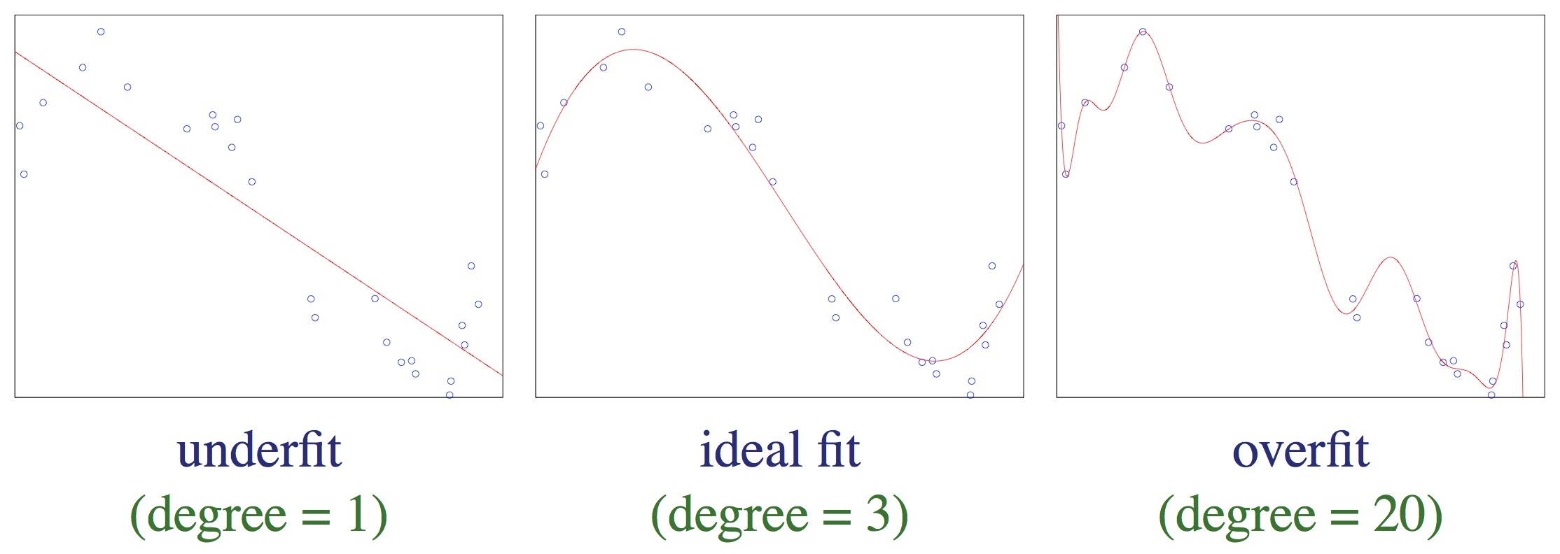
Ten model ma duże obciążenie (błąd systematyczny, _bias) – zachodzi niedostateczne dopasowanie (underfitting).

fig = plot_data(X2, y, xlabel="x", ylabel="y")
theta_start = np.matrix([0, 0, 0]).reshape(3, 1)
theta, history = gradient_descent(cost, gradient, theta_start, X2, y, eps=10**-8)
plot_fun(fig, polynomial_regression(theta), X1)
print(f"Koszt: {history[-1][0]}")

Koszt: 0.05470339875188901

Ten model jest odpowiednio dopasowany.

fig = plot_data(X5, y, xlabel="x", ylabel="y")
theta_start = np.matrix([0, 0, 0, 0, 0, 0]).reshape(6, 1)
theta, history = gradient_descent(cost, gradient, theta_start, X5, y, alpha=0.5, eps=10**-8)
plot_fun(fig, polynomial_regression(theta), X1)
print(f"Koszt: {history[-1][0]}")

Koszt: 0.007232337911078077

Ten model ma dużą wariancję (_variance) – zachodzi nadmierne dopasowanie (overfitting).

(Zwróć uwagę na dziwny kształt krzywej w lewej części wykresu – to m.in. efekt nadmiernego dopasowania).

Nadmierne dopasowanie występuje, gdy model ma zbyt dużo stopni swobody w stosunku do ilości danych wejściowych.

Jest to zjawisko niepożądane.

Możemy obrazowo powiedzieć, że nadmierne dopasowanie występuje, gdy model zaczyna modelować szum/zakłócenia w danych zamiast ich „głównego nurtu”.

Zobacz też: https://pl.wikipedia.org/wiki/Nadmierne_dopasowanie

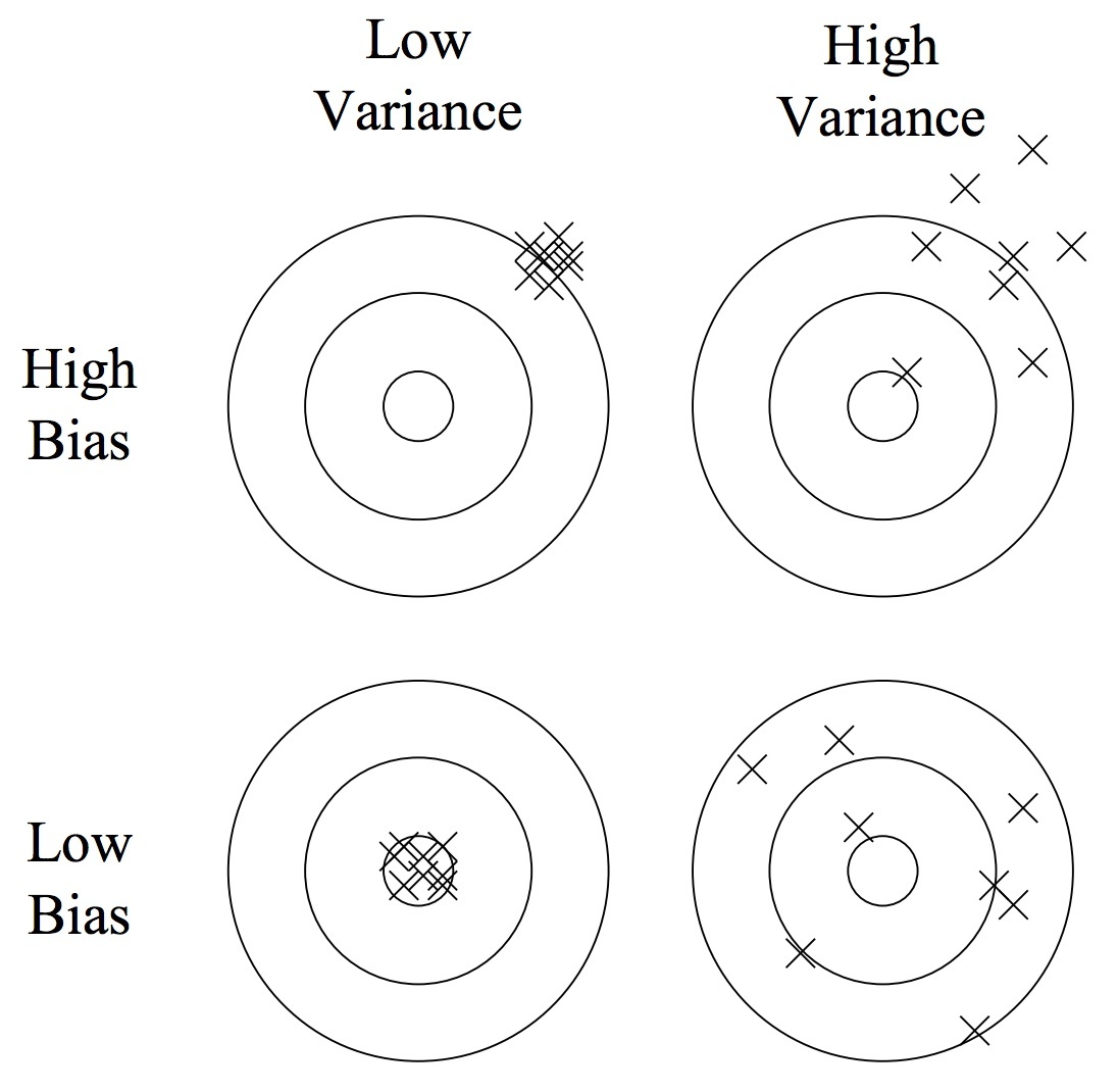
Obciążenie (błąd systematyczny, _bias)

• Wynika z błędnych założeń co do algorytmu uczącego się.
• Duże obciążenie powoduje niedostateczne dopasowanie.

Wariancja (_variance)

• Wynika z nadwrażliwości na niewielkie fluktuacje w zbiorze uczącym.
• Wysoka wariancja może spowodować nadmierne dopasowanie (modelując szum zamiast sygnału).

6.3. Regularyzacja

def SGD(
    h,
    fJ,
    fdJ,
    theta,
    X,
    Y,
    alpha=0.001,
    maxEpochs=1.0,
    batchSize=100,
    adaGrad=False,
    logError=False,
    validate=0.0,
    valStep=100,
    lamb=0,
    trainsetsize=1.0,
):
    """Stochastic Gradient Descent - stochastyczna wersja metody gradientu prostego
    (więcej na ten temat na następnym wykładzie)
    """
    errorsX, errorsY = [], []
    errorsVX, errorsVY = [], []

    XT, YT = X, Y

    m_end = int(trainsetsize * len(X))

    if validate > 0:
        mv = int(X.shape[0] * validate)
        XV, YV = X[:mv], Y[:mv]
        XT, YT = X[mv:m_end], Y[mv:m_end]
    m, n = XT.shape

    start, end = 0, batchSize
    maxSteps = (m * float(maxEpochs)) / batchSize

    if adaGrad:
        hgrad = np.matrix(np.zeros(n)).reshape(n, 1)

    for i in range(int(maxSteps)):
        XBatch, YBatch = XT[start:end, :], YT[start:end, :]

        grad = fdJ(h, theta, XBatch, YBatch, lamb=lamb)
        if adaGrad:
            hgrad += np.multiply(grad, grad)
            Gt = 1.0 / (10**-7 + np.sqrt(hgrad))
            theta = theta - np.multiply(alpha * Gt, grad)
        else:
            theta = theta - alpha * grad

        if logError:
            errorsX.append(float(i * batchSize) / m)
            errorsY.append(fJ(h, theta, XBatch, YBatch).item())
            if validate > 0 and i % valStep == 0:
                errorsVX.append(float(i * batchSize) / m)
                errorsVY.append(fJ(h, theta, XV, YV).item())

        if start + batchSize < m:
            start += batchSize
        else:
            start = 0
        end = min(start + batchSize, m)
    return theta, (errorsX, errorsY, errorsVX, errorsVY)

# Przygotowanie danych do przykładu regularyzacji

n = 6

data = np.matrix(np.loadtxt("ex2data2.txt", delimiter=","))
np.random.shuffle(data)

X = powerme(data[:, 0], data[:, 1], n)
Y = data[:, 2]

def draw_regularization_example(
    X, Y, lamb=0, alpha=1, adaGrad=True, maxEpochs=2500, validate=0.25
):
    """Rusuje przykład regularyzacji"""
    plt.figure(figsize=(16, 8))
    plt.subplot(121)
    plt.scatter(
        X[:, 2].tolist(),
        X[:, 1].tolist(),
        c=Y.tolist(),
        s=100,
        cmap=plt.cm.get_cmap("prism"),
    )

    theta = np.matrix(np.zeros(X.shape[1])).reshape(X.shape[1], 1)
    thetaBest, err = SGD(
        h,
        J,
        dJ,
        theta,
        X,
        Y,
        alpha=alpha,
        adaGrad=adaGrad,
        maxEpochs=maxEpochs,
        batchSize=100,
        logError=True,
        validate=validate,
        valStep=1,
        lamb=lamb,
    )

    xx, yy = np.meshgrid(np.arange(-1.5, 1.5, 0.02), np.arange(-1.5, 1.5, 0.02))
    l = len(xx.ravel())
    C = powerme(xx.reshape(l, 1), yy.reshape(l, 1), n)
    z = classifyBi(thetaBest, C).reshape(int(np.sqrt(l)), int(np.sqrt(l)))

    plt.contour(xx, yy, z, levels=[0.5], lw=3)
    plt.ylim(-1, 1.2)
    plt.xlim(-1, 1.2)
    plt.legend()
    plt.subplot(122)
    plt.plot(err[0], err[1], lw=3, label="Training error")
    if validate > 0:
        plt.plot(err[2], err[3], lw=3, label="Validation error")
    plt.legend()
    plt.ylim(0.2, 0.8)

draw_regularization_example(X, Y)

/tmp/ipykernel_868/2651435526.py:12: MatplotlibDeprecationWarning: The get_cmap function was deprecated in Matplotlib 3.7 and will be removed two minor releases later. Use ``matplotlib.colormaps[name]`` or ``matplotlib.colormaps.get_cmap(obj)`` instead.
  cmap=plt.cm.get_cmap("prism"),
/tmp/ipykernel_868/2678993393.py:5: RuntimeWarning: overflow encountered in exp
  y = 1.0 / (1.0 + np.exp(-x))
/tmp/ipykernel_868/2651435526.py:38: UserWarning: The following kwargs were not used by contour: 'lw'
  plt.contour(xx, yy, z, levels=[0.5], lw=3)
No artists with labels found to put in legend.  Note that artists whose label start with an underscore are ignored when legend() is called with no argument.

Regularyzacja

Regularyzacja jest metodą zapobiegania zjawisku nadmiernego dopasowania (_overfitting) poprzez odpowiednie zmodyfikowanie funkcji kosztu.

Do funkcji kosztu dodawane jest specjalne wyrażenie (wyrażenie regularyzacyjne – zaznaczone na czerwono w poniższych wzorach), będące „karą” za ekstremalne wartości parametrów $\theta$.

W ten sposób preferowane są wektory $\theta$ z mniejszymi wartosciami parametrów – mają automatycznie niższy koszt.

Jak silną regularyzację chcemy zastosować? Możemy o tym zadecydować, dobierajac odpowiednio parametr regularyzacji $\lambda$.

Przedstawiona tu metoda regularyzacji to tzw. metoda L2 (_ridge). Istnieją również inne metody regularyzacji, które charakteryzują się trochę innymi własnościami, np. L2 (lasso) lub elastic net. Więcej na ten temat można przeczytać np. tu:

• L1 and L2 Regularization Methods
• Ridge and Lasso Regression: L1 and L2 Regularization
• Elastic Net Regression

Regularyzacja dla regresji liniowej – funkcja kosztu

$$ J(\theta) , = , \dfrac{1}{2m} \left( \displaystyle\sum_{i=1}^{m} \left( h_\theta(x^{(i)}) - y^{(i)} \right)^2 \color{red}{ + \lambda \displaystyle\sum_{j=1}^{n} \theta^2_j } \right) $$

• $\lambda$ – parametr regularyzacji
• jeżeli $\lambda$ jest zbyt mały, skutkuje to nadmiernym dopasowaniem
• jeżeli $\lambda$ jest zbyt duży, skutkuje to niedostatecznym dopasowaniem

Regularyzacja dla regresji liniowej – gradient

$$\small \begin{array}{llll} \dfrac{\partial J(\theta)}{\partial \theta_0} &=& \dfrac{1}{m}\displaystyle\sum_{i=1}^m \left( h_{\theta}(x^{(i)})-y^{(i)} \right) x^{(i)}_0 & \textrm{dla $j = 0$ }\\ \dfrac{\partial J(\theta)}{\partial \theta_j} &=& \dfrac{1}{m}\displaystyle\sum

Regularyzacja dla regresji logistycznej – funkcja kosztu

$$ \begin{array}{rtl} J(\theta) & = & -\dfrac{1}{m} \left( \displaystyle\sum_{i=1}^{m} y^{(i)} \log h_\theta(x^{(i)}) + \left( 1-y^{(i)} \right) \log \left( 1-h_\theta(x^{(i)}) \right) \right) \\ & & \color{red}{ + \dfrac{\lambda}{2m} \displaystyle\sum_{j=1}^{n} \theta^2_j } \\ \end{array} $$

Regularyzacja dla regresji logistycznej – gradient

$$\small \begin{array}{llll} \dfrac{\partial J(\theta)}{\partial \theta_0} &=& \dfrac{1}{m}\displaystyle\sum_{i=1}^m \left( h_{\theta}(x^{(i)})-y^{(i)} \right) x^{(i)}_0 & \textrm{dla $j = 0$ }\\ \dfrac{\partial J(\theta)}{\partial \theta_j} &=& \dfrac{1}{m}\displaystyle\sum

Implementacja metody regularyzacji

def J_(h, theta, X, y, lamb=0):
    """Funkcja kosztu z regularyzacją"""
    m = float(len(y))
    f = h(theta, X, eps=10**-7)
    j = 1.0 / m * -np.sum(
        np.multiply(y, np.log(f)) + np.multiply(1 - y, np.log(1 - f)), axis=0
    ) + lamb / (2 * m) * np.sum(np.power(theta[1:], 2))
    return j


def dJ_(h, theta, X, y, lamb=0):
    """Gradient funkcji kosztu z regularyzacją"""
    m = float(y.shape[0])
    g = 1.0 / y.shape[0] * (X.T * (h(theta, X) - y))
    g[1:] += lamb / m * theta[1:]
    return g

slider_lambda = widgets.FloatSlider(
    min=0.0, max=0.5, step=0.005, value=0.01, description=r"$\lambda$", width=300
)


def slide_regularization_example_2(lamb):
    draw_regularization_example(X, Y, lamb=lamb)

widgets.interact_manual(slide_regularization_example_2, lamb=slider_lambda)

interactive(children=(FloatSlider(value=0.01, description='$\\\\lambda$', max=0.5, step=0.005), Button(descripti…

<function __main__.slide_regularization_example_2(lamb)>

def cost_lambda_fun(lamb):
    """Koszt w zależności od parametru regularyzacji lambda"""
    theta = np.matrix(np.zeros(X.shape[1])).reshape(X.shape[1], 1)
    thetaBest, err = SGD(
        h,
        J,
        dJ,
        theta,
        X,
        Y,
        alpha=1,
        adaGrad=True,
        maxEpochs=2500,
        batchSize=100,
        logError=True,
        validate=0.25,
        valStep=1,
        lamb=lamb,
    )
    return err[1][-1], err[3][-1]


def plot_cost_lambda():
    """Wykres kosztu w zależności od parametru regularyzacji lambda"""
    plt.figure(figsize=(16, 8))
    ax = plt.subplot(111)
    Lambda = np.arange(0.0, 1.0, 0.01)
    Costs = [cost_lambda_fun(lamb) for lamb in Lambda]
    CostTrain = [cost[0] for cost in Costs]
    CostCV = [cost[1] for cost in Costs]
    plt.plot(Lambda, CostTrain, lw=3, label="training error")
    plt.plot(Lambda, CostCV, lw=3, label="validation error")
    ax.set_xlabel(r"$\lambda$")
    ax.set_ylabel("cost")
    plt.legend()
    plt.ylim(0.2, 0.8)

plot_cost_lambda()

5.4. Krzywa uczenia się

• Krzywa uczenia pozwala sprawdzić, czy uczenie przebiega poprawnie.
• Krzywa uczenia to wykres zależności między wielkością zbioru treningowego a wartością funkcji kosztu.
• Wraz ze wzrostem wielkości zbioru treningowego wartość funkcji kosztu na zbiorze treningowym rośnie.
• Wraz ze wzrostem wielkości zbioru treningowego wartość funkcji kosztu na zbiorze walidacyjnym maleje.

def cost_trainsetsize_fun(m):
    """Koszt w zależności od wielkości zbioru uczącego"""
    theta = np.matrix(np.zeros(X.shape[1])).reshape(X.shape[1], 1)
    thetaBest, err = SGD(
        h,
        J,
        dJ,
        theta,
        X,
        Y,
        alpha=1,
        adaGrad=True,
        maxEpochs=2500,
        batchSize=100,
        logError=True,
        validate=0.25,
        valStep=1,
        lamb=0.01,
        trainsetsize=m,
    )
    return err[1][-1], err[3][-1]


def plot_learning_curve():
    """Wykres krzywej uczenia się"""
    plt.figure(figsize=(16, 8))
    ax = plt.subplot(111)
    M = np.arange(0.3, 1.0, 0.05)
    Costs = [cost_trainsetsize_fun(m) for m in M]
    CostTrain = [cost[0] for cost in Costs]
    CostCV = [cost[1] for cost in Costs]
    plt.plot(M, CostTrain, lw=3, label="training error")
    plt.plot(M, CostCV, lw=3, label="validation error")
    ax.set_xlabel("trainset size")
    ax.set_ylabel("cost")
    plt.legend()

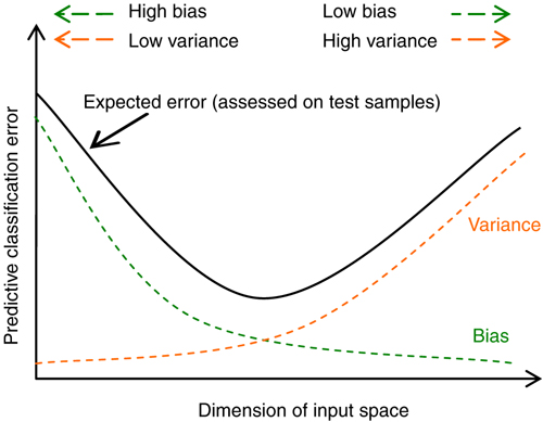
Krzywa uczenia a obciążenie i wariancja

Wykreślenie krzywej uczenia pomaga diagnozować nadmierne i niedostateczne dopasowanie:

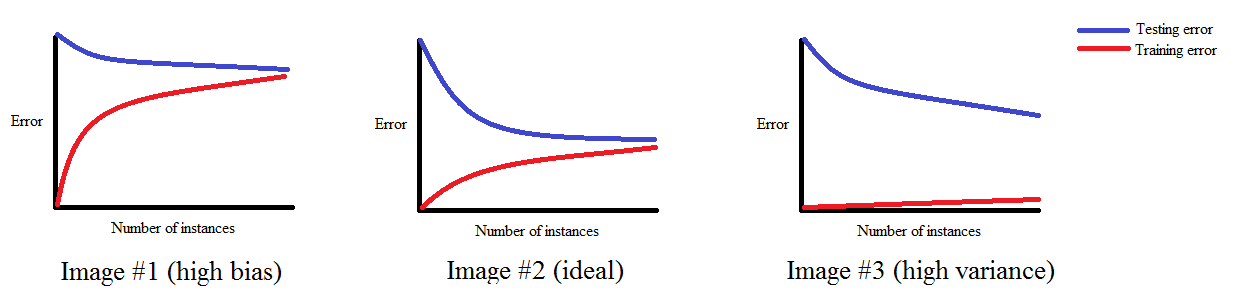
Źródło: http://www.ritchieng.com/machinelearning-learning-curve

plot_learning_curve()