377 KiB
Uczenie maszynowe – zastosowania
5. Regresja wielomianowa. Problem nadmiernego dopasowania
5.1. Regresja wielomianowa
Wprowadzenie: wybór cech
Niech naszym zadaniem będzie przewidzieć cenę działki o kształcie prostokąta.
Jakie cechy wybrać?
Możemy wybrać dwie cechy:
- $x_1$ – szerokość działki, $x_2$ – długość działki: $$ h_{\theta}(\vec{x}) = \theta_0 + \theta_1 x_1 + \theta_2 x_2 $$
...albo jedną:
- $x_1$ – powierzchnia działki: $$ h_{\theta}(\vec{x}) = \theta_0 + \theta_1 x_1 $$
Wniosek: możemy tworzyć nowe cechy na podstawie innych poprzez wykonywanie na nich różnych operacji matematycznych.
Można też zauważyć, że cecha „powierzchnia działki” powstaje przez pomnożenie dwóch innych cech: długości działki i jej szerokości.
Regresja wielomianowa
W regresji wielomianowej będziemy korzystać z cech, które utworzymy jako potęgi cech wyjściowych.
# Przydatne importy

import ipywidgets as widgets
import matplotlib.pyplot as plt
import numpy as np
import pandas

%matplotlib inline
# Przydatne funkcje
def cost(theta, X, y):
"""Wersja macierzowa funkcji kosztu"""
m = len(y)
J = 1.0 / (2.0 * m) * ((X * theta - y).T * (X * theta - y))
return J.item()
def gradient(theta, X, y):
"""Wersja macierzowa gradientu funkcji kosztu"""
return 1.0 / len(y) * (X.T * (X * theta - y))
def gradient_descent(fJ, fdJ, theta, X, y, alpha=0.1, eps=10**-5):
"""Algorytm gradientu prostego (wersja macierzowa)"""
current_cost = fJ(theta, X, y)
logs = [[current_cost, theta]]
while True:
theta = theta - alpha * fdJ(theta, X, y)
current_cost, prev_cost = fJ(theta, X, y), current_cost
if abs(prev_cost - current_cost) > 10**15:
print('Algorithm does not converge!')
break
if abs(prev_cost - current_cost) <= eps:
break
logs.append([current_cost, theta])
return theta, logs
def plot_data(X, y, xlabel, ylabel):
"""Wykres danych (wersja macierzowa)"""
fig = plt.figure(figsize=(16*.6, 9*.6))
ax = fig.add_subplot(111)
fig.subplots_adjust(left=0.1, right=0.9, bottom=0.1, top=0.9)
ax.scatter([X[:, 1]], [y], c='r', s=50, label='Dane')
ax.set_xlabel(xlabel)
ax.set_ylabel(ylabel)
ax.margins(.05, .05)
plt.ylim(y.min() - 1, y.max() + 1)
plt.xlim(np.min(X[:, 1]) - 1, np.max(X[:, 1]) + 1)
return fig
def plot_fun(fig, fun, X):
"""Wykres funkcji `fun`"""
ax = fig.axes[0]
x0 = np.min(X[:, 1]) - 1.0
x1 = np.max(X[:, 1]) + 1.0
Arg = np.arange(x0, x1, 0.1)
Val = fun(Arg)
return ax.plot(Arg, Val, linewidth='2')# Wczytanie danych (mieszkania) przy pomocy biblioteki pandas
alldata = pandas.read_csv('data_flats.tsv', header=0, sep='\t',
usecols=['price', 'rooms', 'sqrMetres'])
data = np.matrix(alldata[['sqrMetres', 'price']])
m, n_plus_1 = data.shape
n = n_plus_1 - 1
Xn = data[:, 0:n]
Xn /= np.amax(Xn, axis=0)
Xn2 = np.power(Xn, 2)
Xn2 /= np.amax(Xn2, axis=0)
Xn3 = np.power(Xn, 3)
Xn3 /= np.amax(Xn3, axis=0)
X = np.matrix(np.concatenate((np.ones((m, 1)), Xn), axis=1)).reshape(m, n + 1)
X2 = np.matrix(np.concatenate((np.ones((m, 1)), Xn, Xn2), axis=1)).reshape(m, 2 * n + 1)
X3 = np.matrix(np.concatenate((np.ones((m, 1)), Xn, Xn2, Xn3), axis=1)).reshape(m, 3 * n + 1)
y = np.matrix(data[:, -1]).reshape(m, 1)Postać ogólna regresji wielomianowej:
$$ h_{\theta}(x) = \sum_{i=0}^{n} \theta_i x^i $$
# Funkcja regresji wielomianowej

def h_poly(Theta, x):
    """Funkcja wielomianowa"""
    return sum(theta * np.power(x, i) for i, theta in enumerate(Theta.tolist()))

def polynomial_regression(theta):
    """Funkcja regresji wielomianowej"""
    return lambda x: h_poly(theta, x)
Najprostszym przypadkiem regresji wielomianowej jest funkcja kwadratowa:
Funkcja kwadratowa:
$$ h_{\theta}(x) = \theta_0 + \theta_1 x + \theta_2 x^2 $$
fig = plot_data(X2, y, xlabel='x', ylabel='y')
theta_start = np.matrix([0, 0, 0]).reshape(3, 1)
theta, logs = gradient_descent(cost, gradient, theta_start, X2, y)
plot_fun(fig, polynomial_regression(theta), X)
[<matplotlib.lines.Line2D at 0x27dd04c6250>]
Innym szczególnym przypadkiem regresji wielomianowej jest funkjca sześcienna:
Funkcja sześcienna:
$$ h_{\theta}(x) = \theta_0 + \theta_1 x + \theta_2 x^2 + \theta_3 x^3 $$
fig = plot_data(X3, y, xlabel='x', ylabel='y')
theta_start = np.matrix([0, 0, 0, 0]).reshape(4, 1)
theta, _ = gradient_descent(cost, gradient, theta_start, X3, y)
plot_fun(fig, polynomial_regression(theta), X)

print(theta)
[[ 397521.22456017] [-841359.33647153] [2253763.58150567] [-244046.90860749]]
Regresję wielomianową można potraktować jako szczególny przypadek regresji liniowej wielu zmiennych:
$$ h_{\theta}(x) = \theta_0 + \theta_1 x + \theta_2 x^2 + \theta_3 x^3 $$ $$ x_1 = x, \quad x_2 = x^2, \quad x_3 = x^3, \quad \vec{x} = \left[ \begin{array}{ccc} x_0 \\ x_1 \\ x_2 \end{array} \right] $$
(W tym przypadku za kolejne cechy przyjmujemy kolejne potęgi zmiennej $x$).
Uwaga praktyczna: przyda się normalizacja cech, szczególnie skalowanie!
Do tworzenia cech „pochodnych” możemy używać nie tylko potęgowania, ale też innych operacji matematycznych, np.:
$$ h_{\theta}(x) = \theta_0 + \theta_1 x + \theta_2 \sqrt{x} $$ $$ x_1 = x, \quad x_2 = \sqrt{x}, \quad \vec{x} = \left[ \begin{array}{ccc} x_0 \\ x_1 \end{array} \right] $$
Jakie zatem cechy wybrać? Najlepiej dopasować je do konkretnego problemu.
Wielomianowa regresja logistyczna
Podobne modyfikacje cech możemy również stosować dla regresji logistycznej.
def powerme(x1,x2,n):
    """Funkcja, która generuje n potęg dla zmiennych x1 i x2 oraz ich iloczynów"""
    X = []
    for m in range(n+1):
        for i in range(m+1):
            X.append(np.multiply(np.power(x1,i),np.power(x2,(m-i))))
    return np.hstack(X)
# Wczytanie danych
import pandas
import numpy as np
alldata = pandas.read_csv('polynomial_logistic.tsv', sep='\t')
data = np.matrix(alldata)
m, n_plus_1 = data.shape
n = n_plus_1 - 1
Xn = data[:, 1:]
Xpl = powerme(data[:, 1], data[:, 2], n)
Ypl = np.matrix(data[:, 0]).reshape(m, 1)
data[:10]matrix([[ 1. , 0.36596696, -0.11214686],
[ 0. , 0.4945305 , 0.47110656],
[ 0. , 0.70290604, -0.92257983],
[ 0. , 0.46658862, -0.62269739],
[ 0. , 0.87939462, -0.11408015],
[ 0. , -0.331185 , 0.84447667],
[ 0. , -0.54351701, 0.8851383 ],
[ 0. , 0.91979241, 0.41607012],
[ 0. , 0.28011742, 0.61431157],
[ 0. , 0.94754363, -0.78307311]])def plot_data_for_classification(X, Y, xlabel, ylabel):
"""Wykres danych (wersja macierzowa)"""
fig = plt.figure(figsize=(16*.6, 9*.6))
ax = fig.add_subplot(111)
fig.subplots_adjust(left=0.1, right=0.9, bottom=0.1, top=0.9)
X = X.tolist()
Y = Y.tolist()
X1n = [x[1] for x, y in zip(X, Y) if y[0] == 0]
X1p = [x[1] for x, y in zip(X, Y) if y[0] == 1]
X2n = [x[2] for x, y in zip(X, Y) if y[0] == 0]
X2p = [x[2] for x, y in zip(X, Y) if y[0] == 1]
ax.scatter(X1n, X2n, c='r', marker='x', s=50, label='Dane')
ax.scatter(X1p, X2p, c='g', marker='o', s=50, label='Dane')
ax.set_xlabel(xlabel)
ax.set_ylabel(ylabel)
ax.margins(.05, .05)
return figPrzyjmijmy, że mamy następujące dane i chcemy przeprowadzić klasyfikację dwuklasową dla następujących klas:
- czerwone krzyżyki
- zielone kółka
fig = plot_data_for_classification(Xpl, Ypl, xlabel=r'$x_1$', ylabel=r'$x_2$')Propozycja hipotezy:
$$ h_\theta(x) = g(\theta^T x) = g(\theta_0 + \theta_1 x_1 + \theta_2 x_2 + \theta_3 x_3 + \theta_4 x_4 + \theta_5 x_5) ; , $$
gdzie $g$ – funkcja logistyczna, $x_3 = x_1^2$, $x_4 = x_2^2$, $x_5 = x_1 x_2$.
def safeSigmoid(x, eps=0):
    """Funkcja sigmoidalna zmodyfikowana w taki sposób,
    żeby wartości zawsz były odległe od asymptot o co najmniej eps
    """
    y = 1.0/(1.0 + np.exp(-x))
    if eps > 0:
        y[y < eps] = eps
        y[y > 1 - eps] = 1 - eps
    return y

def h(theta, X, eps=0.0):
    """Funkcja hipotezy"""
    return safeSigmoid(X*theta, eps)

def J(h,theta,X,y, lamb=0):
    """Funkcja kosztu"""
    m = len(y)
    f = h(theta, X, eps=10**-7)
    j = -np.sum(np.multiply(y, np.log(f)) +
                np.multiply(1 - y, np.log(1 - f)), axis=0)/m
    if lamb > 0:
        j += lamb/(2*m) * np.sum(np.power(theta[1:],2))
    return j

def dJ(h,theta,X,y,lamb=0):
    """Pochodna funkcji kosztu"""
    g = 1.0/y.shape[0]*(X.T*(h(theta,X)-y))
    if lamb > 0:
        g[1:] += lamb/float(y.shape[0]) * theta[1:]
    return g

def classifyBi(theta, X):
    """Funkcja decyzji"""
    prob = h(theta, X)
    return prob
def GD(h, fJ, fdJ, theta, X, y, alpha=0.01, eps=10**-3, maxSteps=10000):
"""Metoda gradientu prostego dla regresji logistycznej"""
errorCurr = fJ(h, theta, X, y)
errors = [[errorCurr, theta]]
while True:
# oblicz nowe theta
theta = theta - alpha * fdJ(h, theta, X, y)
# raportuj poziom błędu
errorCurr, errorPrev = fJ(h, theta, X, y), errorCurr
# kryteria stopu
if abs(errorPrev - errorCurr) <= eps:
break
if len(errors) > maxSteps:
break
errors.append([errorCurr, theta])
return theta, errors# Uruchomienie metody gradientu prostego dla regresji logistycznej
theta_start = np.matrix(np.zeros(Xpl.shape[1])).reshape(Xpl.shape[1],1)
theta, errors = GD(h, J, dJ, theta_start, Xpl, Ypl,
alpha=0.1, eps=10**-7, maxSteps=10000)
print(r'theta = {}'.format(theta))theta = [[ 1.59558981] [ 0.12602307] [ 0.65718518] [-5.26367581] [ 1.96832544] [-6.97946065]]
def plot_decision_boundary(fig, theta, X):
    """Wykres granicy klas"""
    ax = fig.axes[0]
    xx, yy = np.meshgrid(np.arange(-1.0, 1.0, 0.02),
                         np.arange(-1.0, 1.0, 0.02))
    l = len(xx.ravel())
    C = powerme(xx.reshape(l, 1), yy.reshape(l, 1), n)
    z = classifyBi(theta, C).reshape(int(np.sqrt(l)), int(np.sqrt(l)))

    plt.contour(xx, yy, z, levels=[0.5], lw=3);
fig = plot_data_for_classification(Xpl, Ypl, xlabel=r'$x_1$', ylabel=r'$x_2$')
plot_decision_boundary(fig, theta, Xpl)<ipython-input-20-d7e55b0bd73a>:10: UserWarning: The following kwargs were not used by contour: 'lw' plt.contour(xx, yy, z, levels=[0.5], lw=3);
# Wczytanie danych
alldata = pandas.read_csv('polynomial_logistic.tsv', sep='\t')
data = np.matrix(alldata)
m, n_plus_1 = data.shape
Xn = data[:, 1:]
n = 10
Xpl = powerme(data[:, 1], data[:, 2], n)
Ypl = np.matrix(data[:, 0]).reshape(m, 1)
theta_start = np.matrix(np.zeros(Xpl.shape[1])).reshape(Xpl.shape[1],1)
theta, errors = GD(h, J, dJ, theta_start, Xpl, Ypl,
alpha=0.1, eps=10**-7, maxSteps=10000)# Przykład dla większej liczby cech
fig = plot_data_for_classification(Xpl, Ypl, xlabel=r'$x_1$', ylabel=r'$x_2$')
plot_decision_boundary(fig, theta, Xpl)
<ipython-input-20-d7e55b0bd73a>:10: UserWarning: The following kwargs were not used by contour: 'lw' plt.contour(xx, yy, z, levels=[0.5], lw=3);
5.2. Problem nadmiernego dopasowania
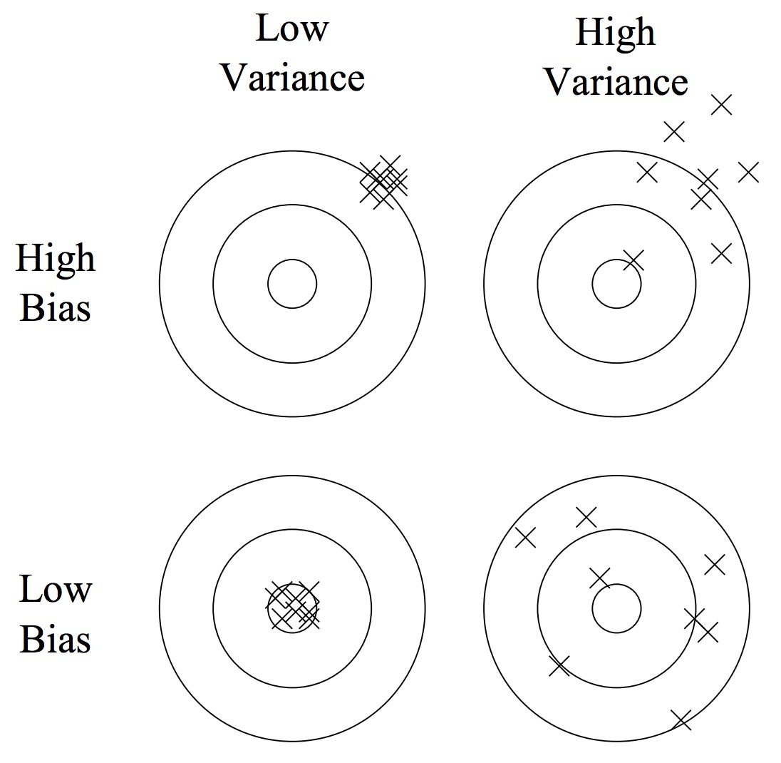
Obciążenie a wariancja
# Dane do prostego przykładu

data = np.matrix([
        [0.0, 0.0],
        [0.5, 1.8],
        [1.0, 4.8],
        [1.6, 7.2],
        [2.6, 8.8],
        [3.0, 9.0],
    ])

m, n_plus_1 = data.shape
n = n_plus_1 - 1
Xn1 = data[:, 0:n]
Xn1 /= np.amax(Xn1, axis=0)
Xn2 = np.power(Xn1, 2)
Xn2 /= np.amax(Xn2, axis=0)
Xn3 = np.power(Xn1, 3)
Xn3 /= np.amax(Xn3, axis=0)
Xn4 = np.power(Xn1, 4)
Xn4 /= np.amax(Xn4, axis=0)
Xn5 = np.power(Xn1, 5)
Xn5 /= np.amax(Xn5, axis=0)

X1 = np.matrix(np.concatenate((np.ones((m, 1)), Xn1), axis=1)).reshape(m, n + 1)
X2 = np.matrix(np.concatenate((np.ones((m, 1)), Xn1, Xn2), axis=1)).reshape(m, 2 * n + 1)
X5 = np.matrix(np.concatenate((np.ones((m, 1)), Xn1, Xn2, Xn3, Xn4, Xn5), axis=1)).reshape(m, 5 * n + 1)
y = np.matrix(data[:, -1]).reshape(m, 1)
fig = plot_data(X1, y, xlabel='x', ylabel='y')fig = plot_data(X1, y, xlabel='x', ylabel='y')
theta_start = np.matrix([0, 0]).reshape(2, 1)
theta, _ = gradient_descent(cost, gradient, theta_start, X1, y, eps=0.00001)
plot_fun(fig, polynomial_regression(theta), X1)[<matplotlib.lines.Line2D at 0x27dd8b81340>]
Ten model ma duże obciążenie (błąd systematyczny, _bias) – zachodzi niedostateczne dopasowanie (underfitting).
fig = plot_data(X2, y, xlabel='x', ylabel='y')
theta_start = np.matrix([0, 0, 0]).reshape(3, 1)
theta, _ = gradient_descent(cost, gradient, theta_start, X2, y, eps=0.000001)
plot_fun(fig, polynomial_regression(theta), X1)
[<matplotlib.lines.Line2D at 0x27e2530e820>]
Ten model jest odpowiednio dopasowany.
fig = plot_data(X5, y, xlabel='x', ylabel='y')
theta_start = np.matrix([0, 0, 0, 0, 0, 0]).reshape(6, 1)
theta, _ = gradient_descent(cost, gradient, theta_start, X5, y, alpha=0.5, eps=10**-7)
plot_fun(fig, polynomial_regression(theta), X1)
[<matplotlib.lines.Line2D at 0x27e250169d0>]
Ten model ma dużą wariancję (_variance) – zachodzi nadmierne dopasowanie (overfitting).
(Zwróć uwagę na dziwny kształt krzywej w lewej części wykresu – to m.in. efekt nadmiernego dopasowania).
Nadmierne dopasowanie występuje, gdy model ma zbyt dużo stopni swobody w stosunku do ilości danych wejściowych.
Jest to zjawisko niepożądane.
Możemy obrazowo powiedzieć, że nadmierne dopasowanie występuje, gdy model zaczyna modelować szum/zakłócenia w danych zamiast ich „głównego nurtu”.

Obciążenie (błąd systematyczny, _bias)
- Wynika z błędnych założeń co do algorytmu uczącego się.
- Duże obciążenie powoduje niedostateczne dopasowanie.
Wariancja (_variance)
- Wynika z nadwrażliwości na niewielkie fluktuacje w zbiorze uczącym.
- Wysoka wariancja może spowodować nadmierne dopasowanie (modelując szum zamiast sygnału).

5.3. Regularyzacja
def SGD(h, fJ, fdJ, theta, X, Y,
        alpha=0.001, maxEpochs=1.0, batchSize=100,
        adaGrad=False, logError=False, validate=0.0, valStep=100, lamb=0, trainsetsize=1.0):
    """Stochastic Gradient Descent - stochastyczna wersja metody gradientu prostego
    (więcej na ten temat na wykładzie 11)
    """
    errorsX, errorsY = [], []
    errorsVX, errorsVY = [], []

    XT, YT = X, Y

    m_end=int(trainsetsize*len(X))

    if validate > 0:
        mv = int(X.shape[0] * validate)
        XV, YV = X[:mv], Y[:mv]
        XT, YT = X[mv:m_end], Y[mv:m_end]
    m, n = XT.shape

    start, end = 0, batchSize
    maxSteps = (m * float(maxEpochs)) / batchSize

    if adaGrad:
        hgrad = np.matrix(np.zeros(n)).reshape(n,1)

    for i in range(int(maxSteps)):
        XBatch, YBatch =  XT[start:end,:], YT[start:end,:]

        grad = fdJ(h, theta, XBatch, YBatch, lamb=lamb)
        if adaGrad:
            hgrad += np.multiply(grad, grad)
            Gt = 1.0 / (10**-7 + np.sqrt(hgrad))
            theta = theta - np.multiply(alpha * Gt, grad)
        else:
            theta = theta - alpha * grad

        if logError:
            errorsX.append(float(i*batchSize)/m)
            errorsY.append(fJ(h, theta, XBatch, YBatch).item())
            if validate > 0 and i % valStep == 0:
                errorsVX.append(float(i*batchSize)/m)
                errorsVY.append(fJ(h, theta, XV, YV).item())

        if start + batchSize < m:
            start += batchSize
        else:
            start = 0
        end = min(start + batchSize, m)
    return theta, (errorsX, errorsY, errorsVX, errorsVY)
# Przygotowanie danych do przykładu regularyzacji
n = 6
data = np.matrix(np.loadtxt("ex2data2.txt", delimiter=","))
np.random.shuffle(data)
X = powerme(data[:,0], data[:,1], n)
Y = data[:,2]def draw_regularization_example(X, Y, lamb=0, alpha=1, adaGrad=True, maxEpochs=2500, validate=0.25):
"""Rusuje przykład regularyzacji"""
plt.figure(figsize=(16,8))
plt.subplot(121)
plt.scatter(X[:, 2].tolist(), X[:, 1].tolist(),
c=Y.tolist(),
s=100, cmap=plt.cm.get_cmap('prism'));
theta = np.matrix(np.zeros(X.shape[1])).reshape(X.shape[1],1)
thetaBest, err = SGD(h, J, dJ, theta, X, Y, alpha=alpha, adaGrad=adaGrad, maxEpochs=maxEpochs, batchSize=100,
logError=True, validate=validate, valStep=1, lamb=lamb)
xx, yy = np.meshgrid(np.arange(-1.5, 1.5, 0.02),
np.arange(-1.5, 1.5, 0.02))
l = len(xx.ravel())
C = powerme(xx.reshape(l, 1),yy.reshape(l, 1), n)
z = classifyBi(thetaBest, C).reshape(int(np.sqrt(l)), int(np.sqrt(l)))
plt.contour(xx, yy, z, levels=[0.5], lw=3);
plt.ylim(-1,1.2);
plt.xlim(-1,1.2);
plt.legend();
plt.subplot(122)
plt.plot(err[0],err[1], lw=3, label="Training error")
if validate > 0:
plt.plot(err[2],err[3], lw=3, label="Validation error");
plt.legend()
plt.ylim(0.2,0.8);draw_regularization_example(X, Y)<ipython-input-17-7e1d5e247279>:5: RuntimeWarning: overflow encountered in exp y = 1.0/(1.0 + np.exp(-x)) <ipython-input-31-f0220c89a5e3>:19: UserWarning: The following kwargs were not used by contour: 'lw' plt.contour(xx, yy, z, levels=[0.5], lw=3); No handles with labels found to put in legend.
Regularyzacja
Regularyzacja jest metodą zapobiegania zjawisku nadmiernego dopasowania (_overfitting) poprzez odpowiednie zmodyfikowanie funkcji kosztu.
Do funkcji kosztu dodawane jest specjalne wyrażenie (wyrazenie regularyzacyjne – zaznaczone na czerwono w poniższych wzorach), będące „karą” za ekstremalne wartości parametrów $\theta$.
W ten sposób preferowane są wektory $\theta$ z mniejszymi wartosciami parametrów – mają automatycznie niższy koszt.
Jak silną regularyzację chcemy zastosować? Możemy o tym zadecydować, dobierajac odpowiednio parametr regularyzacji $\lambda$.
Regularyzacja dla regresji liniowej – funkcja kosztu
$$ J(\theta) , = , \dfrac{1}{2m} \left( \displaystyle\sum_{i=1}^{m} \left( h_\theta(x^{(i)}) - y^{(i)} \right) \color{red}{ + \lambda \displaystyle\sum_{j=1}^{n} \theta^2_j } \right) $$
- $\lambda$ – parametr regularyzacji
- jeżeli $\lambda$ jest zbyt mały, skutkuje to nadmiernym dopasowaniem
- jeżeli $\lambda$ jest zbyt duży, skutkuje to niedostatecznym dopasowaniem
Regularyzacja dla regresji liniowej – gradient
$$\small \begin{array}{llll} \dfrac{\partial J(\theta)}{\partial \theta_0} &=& \dfrac{1}{m}\displaystyle\sum_{i=1}^m \left( h_{\theta}(x^{(i)})-y^{(i)} \right) x^{(i)}_0 & \textrm{dla $j = 0$ }\\ \dfrac{\partial J(\theta)}{\partial \theta_j} &=& \dfrac{1}{m}\displaystyle\sum
Regularyzacja dla regresji logistycznej – funkcja kosztu
$$ \begin{array}{rtl} J(\theta) & = & -\dfrac{1}{m} \left( \displaystyle\sum_{i=1}^{m} y^{(i)} \log h_\theta(x^{(i)}) + \left( 1-y^{(i)} \right) \log \left( 1-h_\theta(x^{(i)}) \right) \right) \\ & & \color{red}{ + \dfrac{\lambda}{2m} \displaystyle\sum_{j=1}^{n} \theta^2_j } \\ \end{array} $$
Regularyzacja dla regresji logistycznej – gradient
$$\small \begin{array}{llll} \dfrac{\partial J(\theta)}{\partial \theta_0} &=& \dfrac{1}{m}\displaystyle\sum_{i=1}^m \left( h_{\theta}(x^{(i)})-y^{(i)} \right) x^{(i)}_0 & \textrm{dla $j = 0$ }\\ \dfrac{\partial J(\theta)}{\partial \theta_j} &=& \dfrac{1}{m}\displaystyle\sum
Implementacja metody regularyzacji
def J_(h,theta,X,y,lamb=0):
    """Funkcja kosztu z regularyzacją"""
    m = float(len(y))
    f = h(theta, X, eps=10**-7)
    j = 1.0/m \
        * -np.sum(np.multiply(y, np.log(f)) +
                  np.multiply(1 - y, np.log(1 - f)), axis=0) \
        + lamb/(2*m) * np.sum(np.power(theta[1:] ,2))
    return j

def dJ_(h,theta,X,y,lamb=0):
    """Gradient funkcji kosztu z regularyzacją"""
    m = float(y.shape[0])
    g = 1.0/y.shape[0]*(X.T*(h(theta,X)-y))
    g[1:] += lamb/m * theta[1:]
    return g
slider_lambda = widgets.FloatSlider(min=0.0, max=0.5, step=0.005, value=0.01, description=r'$\lambda$', width=300)
def slide_regularization_example_2(lamb):
draw_regularization_example(X, Y, lamb=lamb)widgets.interact_manual(slide_regularization_example_2, lamb=slider_lambda)interactive(children=(FloatSlider(value=0.01, description='$\\\\lambda$', max=0.5, step=0.005), Button(descripti…
<function __main__.slide_regularization_example_2(lamb)>
def cost_lambda_fun(lamb):
    """Koszt w zależności od parametru regularyzacji lambda"""
    theta = np.matrix(np.zeros(X.shape[1])).reshape(X.shape[1],1)
    thetaBest, err = SGD(h, J, dJ, theta, X, Y, alpha=1, adaGrad=True, maxEpochs=2500, batchSize=100,
                         logError=True, validate=0.25, valStep=1, lamb=lamb)
    return err[1][-1], err[3][-1]

def plot_cost_lambda():
    """Wykres kosztu w zależności od parametru regularyzacji lambda"""
    plt.figure(figsize=(16,8))
    ax = plt.subplot(111)
    Lambda = np.arange(0.0, 1.0, 0.01)
    Costs = [cost_lambda_fun(lamb) for lamb in Lambda]
    CostTrain = [cost[0] for cost in Costs]
    CostCV = [cost[1] for cost in Costs]
    plt.plot(Lambda, CostTrain, lw=3, label='training error')
    plt.plot(Lambda, CostCV, lw=3, label='validation error')
    ax.set_xlabel(r'$\lambda$')
    ax.set_ylabel(u'cost')
    plt.legend()
plt.ylim(0.2,0.8)plot_cost_lambda()5.4. Krzywa uczenia się
- Krzywa uczenia pozwala sprawdzić, czy uczenie przebiega poprawnie.
- Krzywa uczenia to wykres zależności między wielkością zbioru treningowego a wartością funkcji kosztu.
- Wraz ze wzrostem wielkości zbioru treningowego wartość funkcji kosztu na zbiorze treningowym rośnie.
- Wraz ze wzrostem wielkości zbioru treningowego wartość funkcji kosztu na zbiorze walidacyjnym maleje.
def cost_trainsetsize_fun(m):
    """Koszt w zależności od wielkości zbioru uczącego"""
    theta = np.matrix(np.zeros(X.shape[1])).reshape(X.shape[1],1)
    thetaBest, err = SGD(h, J, dJ, theta, X, Y, alpha=1, adaGrad=True, maxEpochs=2500, batchSize=100,
                         logError=True, validate=0.25, valStep=1, lamb=0.01, trainsetsize=m)
    return err[1][-1], err[3][-1]

def plot_learning_curve():
    """Wykres krzywej uczenia się"""
    plt.figure(figsize=(16,8))
    ax = plt.subplot(111)
    M = np.arange(0.3, 1.0, 0.05)
    Costs = [cost_trainsetsize_fun(m) for m in M]
    CostTrain = [cost[0] for cost in Costs]
    CostCV = [cost[1] for cost in Costs]
    plt.plot(M, CostTrain, lw=3, label='training error')
    plt.plot(M, CostCV, lw=3, label='validation error')
    ax.set_xlabel(u'trainset size')
    ax.set_ylabel(u'cost')
    plt.legend()
Krzywa uczenia a obciążenie i wariancja
Wykreślenie krzywej uczenia pomaga diagnozować nadmierne i niedostateczne dopasowanie:
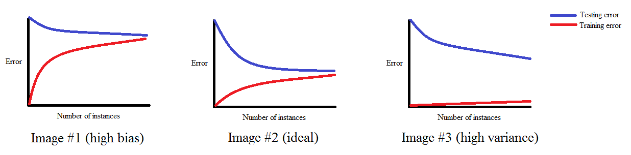
Źródło: http://www.ritchieng.com/machinelearning-learning-curve
plot_learning_curve()