Regresja wielomianowa

Celem regresji wielomianowej jest zamodelowanie relacji między zmienną zależną od zmiennych niezależnych jako funkcję wielomianu n-tego stopnia.

Postać ogólna regresji wielomianowej:

$$ h_{\theta}(x) = \sum_{i=0}^{n} \theta_i x^i $$

Gdzie:

$$ \theta - \text{wektor parametrów modelu} $$

Funkcja kosztu

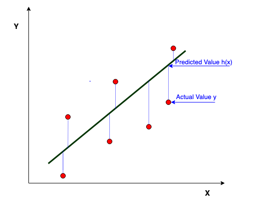
W celu odpowiedniego dobrania parametrów modelu, trzeba znaleźć minimum funkcji kosztu zdefiniowanej poniższym wzorem:

$$ J = \frac{1}{2m} (X \theta - y)^T (X \theta - y) $$

Gdzie:

$$ m - \text{ilość przykładów} $$

Za funkcję kosztu przyjmuje się zmodyfikowaną wersję błędu średniokwadratowego. Dodatkowo dodaje się dzielenie przez 2*m zamiast m, aby gradient z funkcji był lepszej postaci.

Metoda gradientu prostego

Do znalezienia minimum funckji kosztu można użyć metody gradientu prostego. W tym celu iteracyjnie liczy się gradient funkcji kosztu i aktualizuje się za jego pomocą wektor parametrów modelu aż do uzyskania zbieżności (Różnica między obliczoną funkcją kosztu a funkcją kosztu w poprzedniej iteracji będzie mniejsza od ustalonej wcześniej wartości $\varepsilon$).

Gradient funkcji kosztu:

$$ \dfrac{\partial J(\theta)}{\partial \theta} = \frac{1}{m}X^T(X \theta - y)$$

Modyfikacja parametrów modelu:

$$ \theta_{new} = \theta - \alpha * \dfrac{\partial J(\theta)}{\partial \theta}$$

Gdzie:

$$ \alpha - \text{współczynnik uczenia} $$

import ipywidgets as widgets
import matplotlib.pyplot as plt
import numpy as np
import pandas

%matplotlib inline

# Przydatne funkcje
cost_functions = dict()

def cost(theta, X, y):
    """Wersja macierzowa funkcji kosztu"""
    m = len(y)
    J = 1.0 / (2.0 * m) * ((X * theta - y).T * (X * theta - y))
    return J.item()

def gradient(theta, X, y):
    """Wersja macierzowa gradientu funkcji kosztu"""
    return 1.0 / len(y) * (X.T * (X * theta - y)) 

def gradient_descent(fJ, fdJ, theta, X, y, alpha=0.1, eps=10**-7):
    """Algorytm gradientu prostego"""
    current_cost = fJ(theta, X, y)
    logs = [[current_cost, theta]]
    while True:
        theta = theta - alpha * fdJ(theta, X, y)
        current_cost, prev_cost = fJ(theta, X, y), current_cost
        # print(current_cost)
        if abs(prev_cost - current_cost) > 10**15:
            print('Algorytm nie jest zbieżny!')
            break
        if abs(prev_cost - current_cost) <= eps:
            break
        logs.append([current_cost, theta]) 
    return theta, logs

def plot_data(X, y, xlabel, ylabel):
    """Wykres danych"""
    fig = plt.figure(figsize=(16*.6, 9*.6))
    ax = fig.add_subplot(111)
    fig.subplots_adjust(left=0.1, right=0.9, bottom=0.1, top=0.9)
    ax.scatter([X[:, 1]], [y], c='r', s=50, label='Dane')
    
    ax.set_xlabel(xlabel)
    ax.set_ylabel(ylabel)
    ax.margins(.05, .05)
    plt.ylim(y.min() - 1, y.max() + 1)
    plt.xlim(np.min(X[:, 1]) - 1, np.max(X[:, 1]) + 1)
    return fig

def plot_data_cost(X, y, xlabel, ylabel):
    """Wykres funkcji kosztu"""
    fig = plt.figure(figsize=(16 * .6, 9 * .6))
    ax = fig.add_subplot(111)
    fig.subplots_adjust(left=0.1, right=0.9, bottom=0.1, top=0.9)
    ax.scatter([X], [y], c='r', s=50, label='Dane')

    ax.set_xlabel(xlabel)
    ax.set_ylabel(ylabel)
    ax.margins(.05, .05)
    plt.ylim(min(y) - 1, max(y) + 1)
    plt.xlim(np.min(X) - 1, np.max(X) + 1)
    return fig

def plot_fun(fig, fun, X):
    """Wykres funkcji `fun`"""
    ax = fig.axes[0]
    x0 = np.min(X[:, 1]) - 1.0
    x1 = np.max(X[:, 1]) + 1.0
    Arg = np.arange(x0, x1, 0.1)
    Val = fun(Arg)
    return ax.plot(Arg, Val, linewidth='2')

def MSE(Y_true, Y_pred):
    """Błąd średniokwadratowy - Mean Squared Error"""
    return np.square(np.subtract(Y_true,Y_pred)).mean()

# Funkcja regresji wielomianowej

def h_poly(Theta, x):
    """Funkcja wielomianowa"""
    return sum(theta * np.power(x, i) for i, theta in enumerate(Theta.tolist()))

def get_poly_data(data, deg):
    """Przygotowanie danych do regresji wielomianowej"""
    m, n_plus_1 = data.shape
    n = n_plus_1 - 1

    X1 = data[:, 0:n]
    X1 /= np.amax(X1, axis=0)

    Xs = [np.ones((m, 1)), X1]

    for i in range(2, deg+1):
        Xn = np.power(X1, i)
        Xn /= np.amax(Xn, axis=0)
        Xs.append(Xn)

    X = np.matrix(np.concatenate(Xs, axis=1)).reshape(m, deg * n + 1)

    y = np.matrix(data[:, -1]).reshape(m, 1)

    return X, y


def polynomial_regression(X, y, n):
    """Funkcja regresji wielomianowej"""
    theta_start = np.matrix([0] * (n+1)).reshape(n+1, 1)
    theta, logs = gradient_descent(cost, gradient, theta_start, X, y)
    return lambda x: h_poly(theta, x), logs

def predict_values(model, data, n):
    """Funkcja predykcji"""
    x, y = get_poly_data(np.array(data), n)
    preprocessed_x = []
    for i in x:
        preprocessed_x.append(i.item(1))
    return y, model(preprocessed_x), MSE(y, model(preprocessed_x))

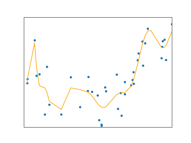
def plot_and_mse(data, data_test, n):
    """Wykres wraz z MSE"""
    x, y = get_poly_data(np.array(data), n)
    model, logs = polynomial_regression(x, y, n)
    cost_function = [[element[0], i] for i, element in enumerate(logs)]
    cost_functions[n] = cost_function
    
    fig = plot_data(x, y, xlabel='x', ylabel='y')
    plot_fun(fig, model, x)

    y_true, Y_pred, mse = predict_values(model, data_test, n)
    print(f'Wielomian {n} stopnia, MSE = {mse}')

# Wczytanie danych (mieszkania) przy pomocy biblioteki pandas

alldata = pandas.read_csv('data_flats.tsv', header=0, sep='\t',
                          usecols=['price', 'rooms', 'sqrMetres'])
alldata = alldata[['sqrMetres', 'price']]
alldata = alldata.sample(frac=1)
alldata

	sqrMetres	price
651	40	245832.0
1254	35	180000.0
1183	92	429000.0
1196	54	156085.0
1463	62	339282.0
...	...	...
994	33	207000.0
657	74	400000.0
1365	55	535000.0
934	72	430000.0
546	120	535000.0

1674 rows × 2 columns

# alldata = np.matrix(alldata[['sqrMetres', 'price']])
data_train = alldata[0:1600]
data_test = alldata[1600:]
data_train = np.matrix(data_train).astype(float)
data_test = np.matrix(data_test).astype(float)

cost_fun_slices = []
for n in range(1, 4):
    plot_and_mse(data_train, data_test, n)
    
    cost_data = cost_functions.get(n)
    cost_x = [line[1] for line in cost_data[:250]]
    cost_y = [line[0] for line in cost_data[:250]]
    cost_fun_slices.append((cost_x, cost_y))

Wielomian 1 stopnia, MSE = 40830919432.83225
Wielomian 2 stopnia, MSE = 87109963962.58508
Wielomian 3 stopnia, MSE = 86319119164.94438

#WYKRESY FUNKCJI KOSZTU
for fig in cost_fun_slices:
    cost_x, cost_y = fig
    fig = plot_data_cost(cost_x, cost_y, "Iteration", "Cost function value")

# Wczytanie danych przy pomocy biblioteki pandas

alldata_p2 = pandas.read_csv('polynomial-regression_2.csv')
alldata_p2 = alldata_p2.sample(frac=1)
alldata_p2

	araba_fiyat	araba_max_hiz
3	100	200
1	70	180
11	750	360
8	300	300
6	200	240
5	150	220
13	2000	365
7	250	240
9	400	350
0	60	180
12	1000	365
10	500	350
4	120	200
14	3000	365
2	80	200

# alldata = np.matrix(alldata[['sqrMetres', 'price']])
data_train_p2 = alldata_p2[0:12]
data_test_p2 = alldata_p2[12:]
data_train_p2 = np.matrix(data_train_p2).astype(float)
data_test_p2 = np.matrix(data_test_p2).astype(float)

cost_fun_slices = []
for n in range(1, 4):
    plot_and_mse(data_train_p2, data_test_p2, n)
    
    cost_data = cost_functions.get(n)
    cost_x = [line[1] for line in cost_data[:250]]
    cost_y = [line[0] for line in cost_data[:250]]
    cost_fun_slices.append((cost_x, cost_y))

Wielomian 1 stopnia, MSE = 16499.91920339438
Wielomian 2 stopnia, MSE = 11862.306362249277
Wielomian 3 stopnia, MSE = 14326.050185115093

#WYKRESY FUNKCJI KOSZTU
for fig in cost_fun_slices:
    cost_x, cost_y = fig
    fig = plot_data_cost(cost_x, cost_y, "Iteration", "Cost function value")

# Ilość nauki do oceny

data_marks_all = pandas.read_csv('Student_Marks.csv')
data_marks_all

	number_courses	time_study	Marks
0	3	4.508	19.202
1	4	0.096	7.734
2	4	3.133	13.811
3	6	7.909	53.018
4	8	7.811	55.299
...	...	...	...
95	6	3.561	19.128
96	3	0.301	5.609
97	4	7.163	41.444
98	7	0.309	12.027
99	3	6.335	32.357

100 rows × 3 columns

data_marks_all = data_marks_all[['time_study', 'Marks']]
# data_marks_all = data_marks_all.sample(frac=1)
data_marks_train = data_marks_all[0:70]
data_marks_test = data_marks_all[70:]
data_marks_train = np.matrix(data_marks_train).astype(float)
data_marks_test = np.matrix(data_marks_test).astype(float)

cost_fun_slices = []

for n in range(1, 4):
    plot_and_mse(data_marks_train, data_marks_test, n)
    
    cost_data = cost_functions.get(n)
    cost_x = [line[1] for line in cost_data[:250]]
    cost_y = [line[0] for line in cost_data[:250]]
    cost_fun_slices.append((cost_x, cost_y))

Wielomian 1 stopnia, MSE = 381.16937283505433
Wielomian 2 stopnia, MSE = 394.1863119057109
Wielomian 3 stopnia, MSE = 391.5017110730558

#WYKRESY FUNKCJI KOSZTU
for fig in cost_fun_slices:
    cost_x, cost_y = fig
    fig = plot_data_cost(cost_x, cost_y, "Iteration", "Cost function value")

data_ins = pandas.read_csv('insurance.csv')
data_ins = data_ins.sample(frac=1)
data_ins

	age	sex	bmi	children	smoker	region	charges
949	25	male	29.700	3	yes	southwest	19933.45800
166	20	female	37.000	5	no	southwest	4830.63000
365	49	female	30.780	1	no	northeast	9778.34720
1183	48	female	27.360	1	no	northeast	9447.38240
772	44	female	36.480	0	no	northeast	12797.20962
...	...	...	...	...	...	...	...
1205	35	male	17.860	1	no	northwest	5116.50040
158	30	male	35.530	0	yes	southeast	36950.25670
740	45	male	24.035	2	no	northeast	8604.48365
907	44	female	32.340	1	no	southeast	7633.72060
1162	30	male	38.830	1	no	southeast	18963.17192

1338 rows × 7 columns

data_ins = data_ins[['age', 'charges']]
data_ins_train = data_ins[0:1200]
data_ins_test = data_ins[1200:]
data_ins_train = np.matrix(data_ins_train).astype(float)
data_ins_test = np.matrix(data_ins_test).astype(float)

cost_fun_slices = []

for n in range(1, 4):
    plot_and_mse(data_ins_train, data_ins_test, n)
    
    cost_data = cost_functions.get(n)
    cost_x = [line[1] for line in cost_data[:250]]
    cost_y = [line[0] for line in cost_data[:250]]
    cost_fun_slices.append((cost_x, cost_y))

Wielomian 1 stopnia, MSE = 183212045.05222273
Wielomian 2 stopnia, MSE = 183706365.10358346
Wielomian 3 stopnia, MSE = 183691092.4723696

#WYKRESY FUNKCJI KOSZTU
for fig in cost_fun_slices:
    cost_x, cost_y = fig
    fig = plot_data_cost(cost_x, cost_y, "Iteration", "Cost function value")

478 KiB Raw Blame History Unescape Escape

Regresja wielomianowa

Funkcja kosztu

Metoda gradientu prostego

478 KiB

Raw Blame History